How Does An Increase In Interest Rate Affect The Is Curve?

16.25 The IS-LM Model

The IS-LM model provides another style of looking at the determination of the level of short-run real gross domestic production (real GDP) in the economy. Like the amass expenditure model, it takes the toll level as fixed. Just whereas that model takes the interest rate as exogenous—specifically, a change in the interest charge per unit results in a change in autonomous spending—the IS-LM model treats the interest rate as an endogenous variable.

The basis of the IS-LM model is an analysis of the coin market and an analysis of the appurtenances market, which together determine the equilibrium levels of interest rates and output in the economy, given prices. The model finds combinations of involvement rates and output (Gross domestic product) such that the money market is in equilibrium. This creates the LM curve. The model too finds combinations of involvement rates and output such that the appurtenances market is in equilibrium. This creates the IS bend. The equilibrium is the interest rate and output combination that is on both the IS and the LM curves.

LM Curve

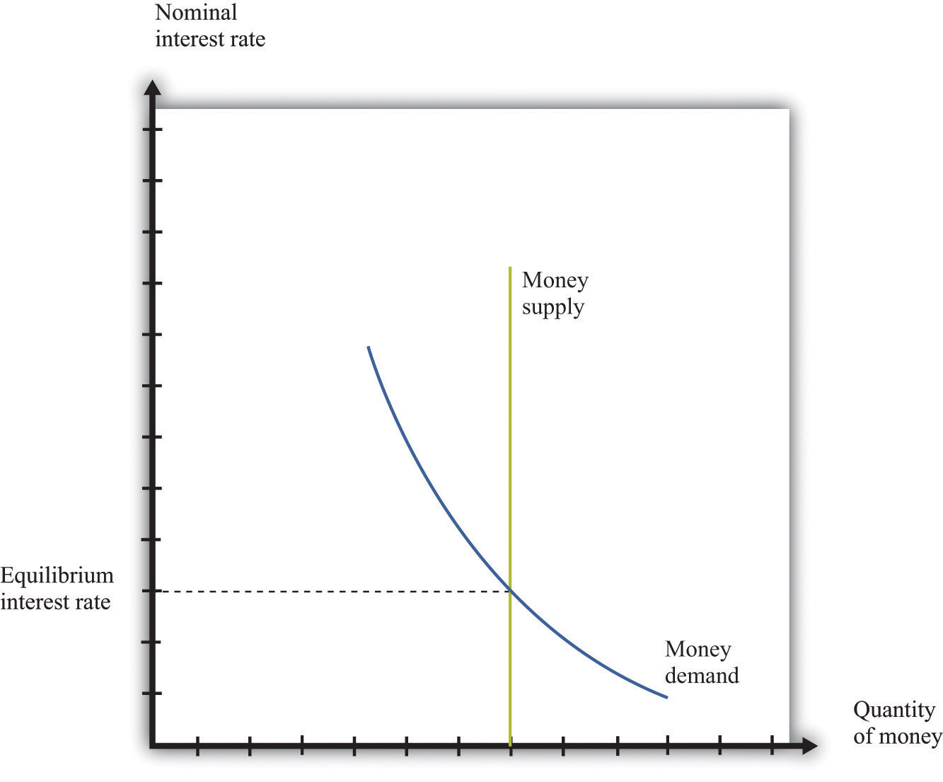
The LM bend represents the combinations of the interest rate and income such that coin supply and money demand are equal. The need for coin comes from households, firms, and governments that employ money as a means of commutation and a store of value. The constabulary of need holds: as the interest rate increases, the quantity of money demanded decreases considering the interest rate represents an opportunity cost of holding money. When involvement rates are college, in other words, money is less effective as a store of value.

Coin demand increases when output rises considering money also serves as a medium of exchange. When output is larger, people have more income and then want to concord more coin for their transactions.

The supply of coin is called by the monetary authority and is contained of the interest rate. Thus it is drawn as a vertical line. The equilibrium in the money market is shown in Figure 16.17 "Coin Market Equilibrium". When the money supply is chosen by the monetary authority, the interest rate is the price that brings the market into equilibrium. Sometimes, in some countries, central banks target the money supply. Alternatively, key banks may choose to target the interest rate. (This was the case we considered in Affiliate 10 "Understanding the Fed".) Figure 16.17 "Coin Market Equilibrium" applies in either example: if the budgetary authorization targets the interest rate, then the money market tells us what the level of the coin supply must be.

Figure xvi.17 Money Marketplace Equilibrium

To trace out the LM bend, nosotros look at what happens to the involvement rate when the level of output in the economic system changes and the supply of money is held fixed. Figure sixteen.18 "A Alter in Income" shows the money marketplace equilibrium at two different levels of real GDP. At the higher level of income, coin need is shifted to the right; the interest charge per unit increases to ensure that coin demand equals money supply. Thus the LM curve is upward sloping: higher real Gdp is associated with college interest rates. At each betoken along the LM bend, money supply equals money need.

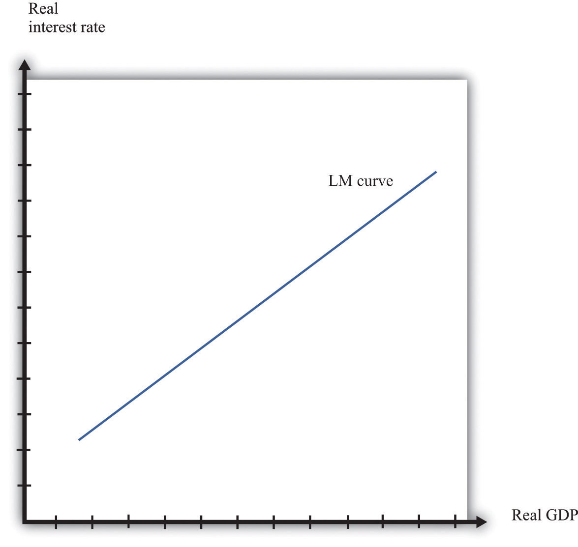
We have not withal been specific about whether nosotros are talking about nominal interest rates or real interest rates. In fact, information technology is the nominal involvement rate that represents the opportunity toll of holding coin. When we draw the LM curve, notwithstanding, we put the real interest charge per unit on the axis, equally shown in Figure sixteen.19 "The LM Curve". The simplest way to recall about this is to suppose that we are because an economy where the aggrandizement charge per unit is zero. In this case, by the Fisher equation, the nominal and existent interest rates are the same. In a more complete analysis, nosotros can comprise aggrandizement past noting that changes in the inflation rate volition shift the LM bend. Changes in the money supply also shift the LM curve.

Figure 16.18 A Change in Income

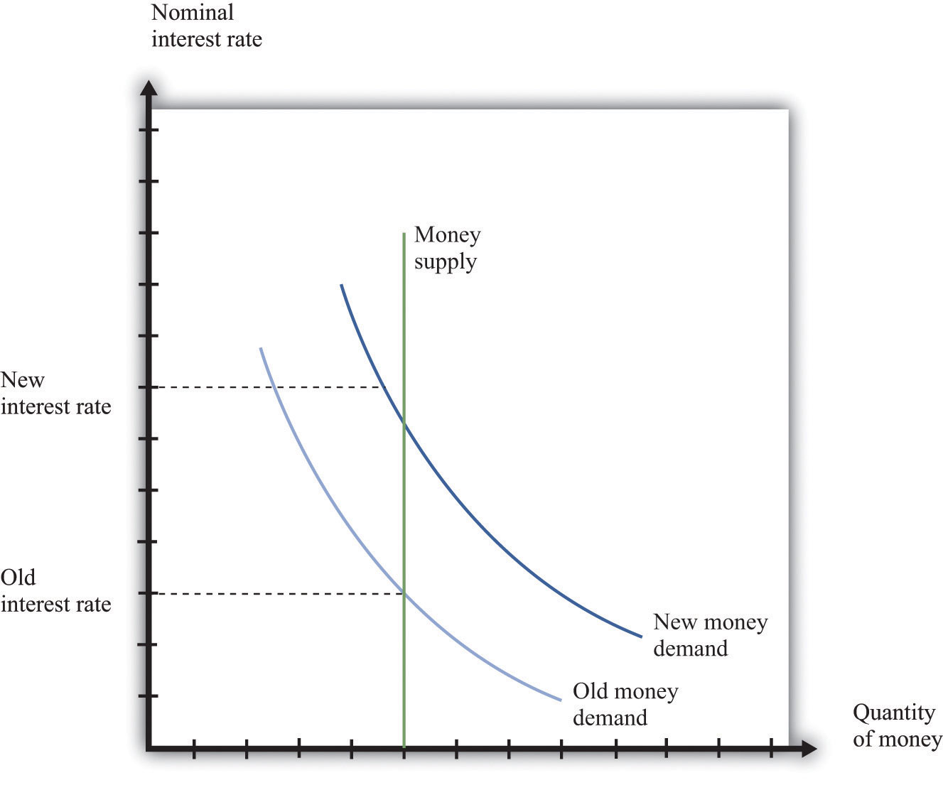
Figure 16.19 The LM Bend

IS Bend

The IS curve relates the level of real Gdp and the real involvement rate. It incorporates both the dependence of spending on the existent involvement rate and the fact that, in the short run, real Gross domestic product equals spending. The IS curve is shown in Figure 16.18 "A Modify in Income". We label the horizontal axis "real GDP" since, in the brusque run, real GDP is adamant by aggregate spending. The IS curve is downward sloping: as the real involvement rate increases, the level of spending decreases.

Effigy sixteen.xx The IS Bend

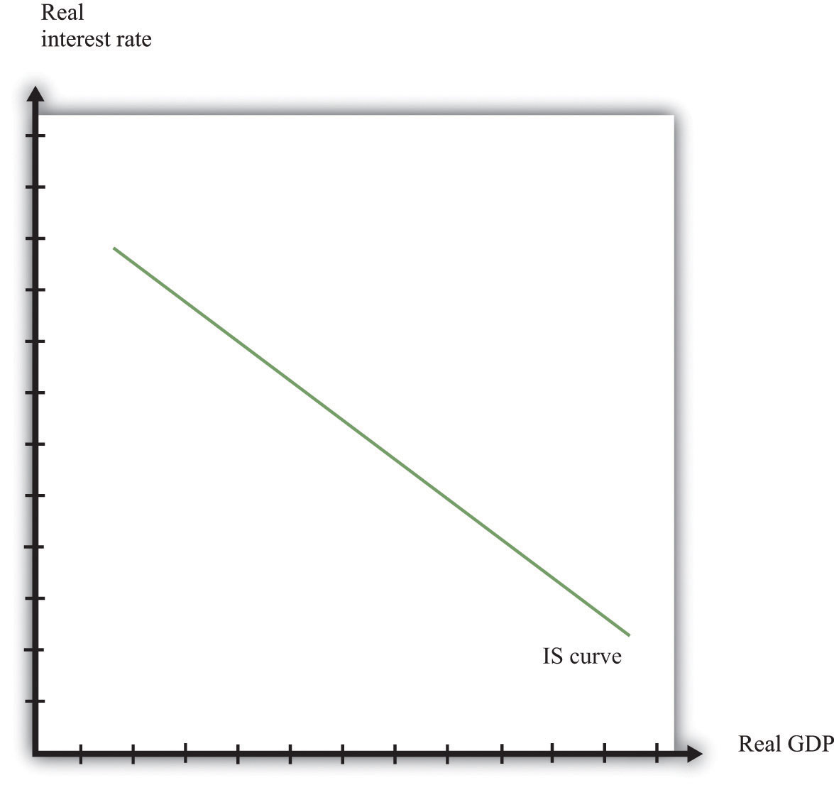
In fact, nosotros derived the IS curve in Affiliate 10 "Understanding the Fed". The dependence of spending on real interest rates comes partly from investment. As the real involvement rate increases, spending by firms on new capital and spending by households on new housing decreases. Consumption also depends on the real involvement rate: spending past households on durable goods decreases as the real interest rate increases.

The connectedness betwixt spending and existent GDP comes from the aggregate expenditure model. Given a item level of the interest rate, the aggregate expenditure model determines the level of real GDP. At present suppose the involvement rate increases. This reduces those components of spending that depend on the interest rate. In the aggregate expenditure framework, this is a reduction in autonomous spending. The equilibrium level of output decreases. Thus the IS curve slopes downwards: college interest rates are associated with lower real Gross domestic product.

Equilibrium

Combining the discussion of the LM and the IS curves will generate equilibrium levels of interest rates and output. Note that both relationships are combinations of interest rates and output. Solving these two equations jointly determines the equilibrium. This is shown graphically in Effigy 16.21. This merely combines the LM curve from Figure 16.19 "The LM Curve" and the IS curve from Effigy sixteen.20 "The IS Curve". The crossing of these ii curves is the combination of the involvement charge per unit and existent Gross domestic product, denoted (r*,Y*), such that both the money marketplace and the goods market are in equilibrium.

Figure 16.21

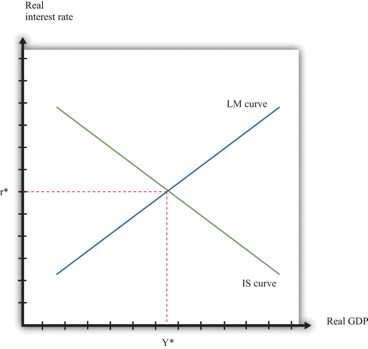
Equilibrium in the IS-LM Model.

Comparative Statics

Comparative statics results for this model illustrate how changes in exogenous factors influence the equilibrium levels of interest rates and output. For this model, at that place are 2 key exogenous factors: the level of democratic spending (excluding any spending affected past involvement rates) and the real money supply. We tin can study how changes in these factors influence the equilibrium levels of output and involvement rates both graphically and algebraically.

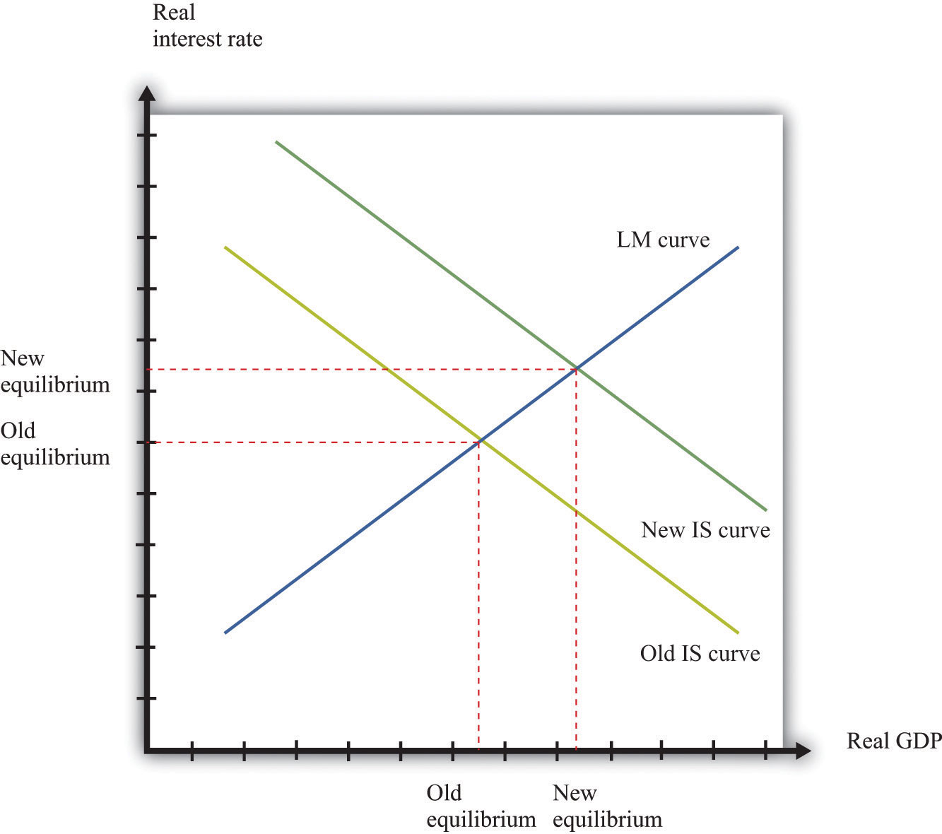
Variations in the level of autonomous spending volition lead to a shift in the IS curve, as shown in Effigy 16.22 "A Shift in the IS Curve". If autonomous spending increases, then the IS bend shifts out. The output level of the economic system volition increment. Interest rates rising as we movement forth the LM bend, ensuring coin market equilibrium. One source of variations in autonomous spending is fiscal policy. Autonomous spending includes government spending (Grand). Thus an increase in G leads to an increase in output and interest rates as shown in Figure sixteen.22 "A Shift in the IS Curve".

Figure sixteen.22 A Shift in the IS Curve

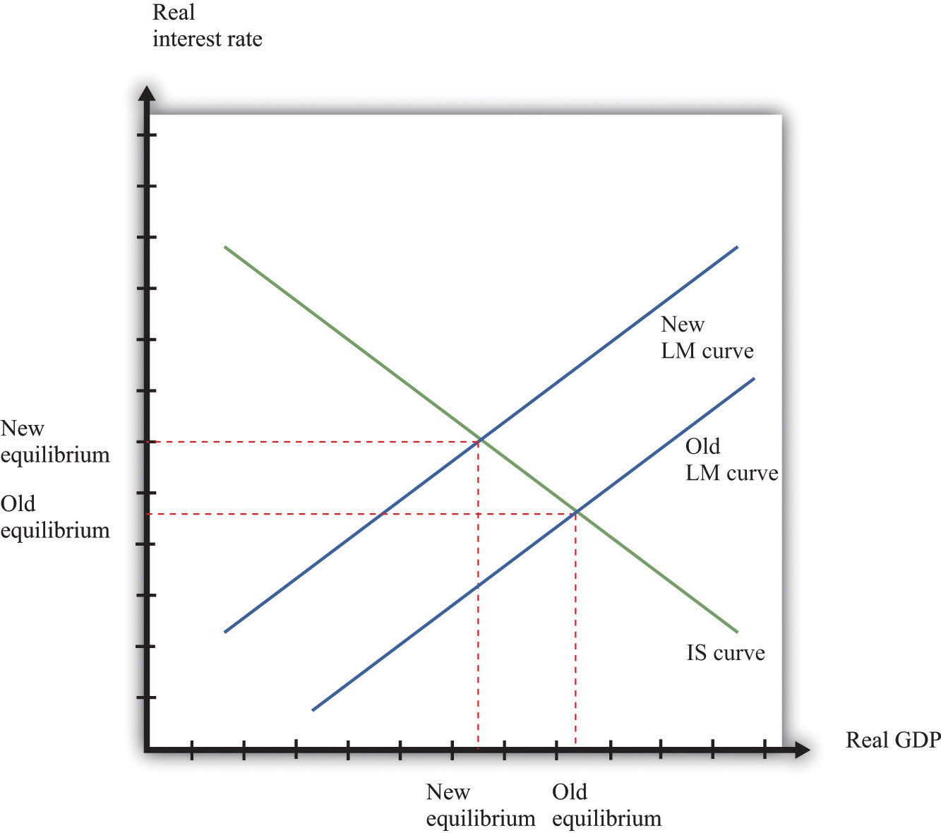
Variations in the existent coin supply shift the LM curve, equally shown in Effigy 16.23 "A Shift in the LM Curve". If the money supply decreases, so the LM curve shifts in. This leads to a higher real involvement rate and lower output every bit the LM curve shifts along the fixed IS curve.

Effigy sixteen.23 A Shift in the LM Bend

More Formally

Nosotros can represent the LM and IS curves algebraically.

LM Curve

Let L(Y,r) stand for real money demand at a level of real GDP of Y and a real involvement rate of r. (When nosotros say "real" coin demand, nosotros mean that, as usual, we have deflated past the price level.) For simplicity, suppose that the inflation rate is cypher, then the real involvement rate is the opportunity price of holding money.If nosotros wanted to include inflation in our analysis, nosotros could write the existent demand for money as 50(Y, r + π), where π is the aggrandizement charge per unit. Assume that real money demand takes a particular form:

L(Y,r) = L₀ + L₁ Y – L₂ r.

In this equation, L₀, L₁, and L₂ are all positive constants. Existent money demand is increasing in income and decreasing in the interest rate. Letting M/P be the real stock of money in the economy, then money marketplace equilibrium requires

1000/P = L₀ + L₁Y – L_two r.

Given a level of real GDP and the existent stock of coin, this equation can be used to solve for the involvement rate such that money supply and money demand are equal. This is given by

r = (one/L₂) [50₀ + L₁Y – Grand/P].

From this equation nosotros learn that an increase in the real stock of money lowers the interest rate, given the level of real GDP. Further, an increase in the level of real Gdp increases the involvement rate, given the stock of money. This is another way of saying that the LM curve is upward sloping.

IS Curve

Recall the 2 equations from the aggregate expenditure model:

Y = E

and

East = E ₀(r) + βY.

Here we take shown explicitly that the level of autonomous spending depends on the real interest charge per unit r.

Nosotros can solve the two equations to notice the values of E and Y that are consistent with both equations. Nosotros notice

$Y^{e q u i l} = (\frac{1}{1 - β}) \times {Eastward}_{0} (r) .$

Given a level of the existent interest rate, we solve for the level of democratic spending (using the dependence of consumption and investment on the real interest rate) so use this equation to find the level of output.

Here is an instance. Suppose that

C = 100 + 0.6Y, I = 400 − vr, G = 300,

and

NX = 200 − 0.iY,

where C is consumption, I is investment, Thousand is government purchases, and NX is net exports. First group the components of spending as follows:

C + I + G + NX = (100 + 400 − fiver + 300 + 200) + (0.sixY − 0.1Y)

Calculation together the first group of terms, nosotros discover autonomous spending:

E ₀ = 100 + 400 + 300 + 200 − 5r = 1000 − vr.

Calculation the coefficients on the income terms, we find the marginal propensity to spend:

β = 0.6 − 0.1 = 0.5.

Using β = 0.5, nosotros summate the multiplier:

$(\frac{ane}{1 - β}) = (\frac{1}{one - . 5}) = two.$

We then summate real Gross domestic product, given the real interest rate:

Y = ii × (m − 5r) = 2000 − 10r.

Equilibrium

Combining the give-and-take of the LM and the IS curves will generate equilibrium levels of interest rates and output. Note that both relationships are combinations of interest rates and output. Solving these 2 equations jointly determines the equilibrium.

Algebraically, we have an equation for the LM curve:

r = (1/L_ii) [L₀ + L_i Y – M/P].

And we have an equation for the IS curve:

Y = mE ₀(r),

where we let m = (1/(ane – β)) denote the multiplier. If we assume that the dependence of spending in the interest charge per unit is linear, so that E ₀(r) = eastward₀ – e₁ r, then the equation for the IS curve is

Y = g (e₀-eastward₁ r),

To solve the IS and LM curves simultaneously, nosotros substitute Y from the IS curve into the LM curve to go

r = (1/Fifty₂) [L₀ + Fifty_ane g(e₀-e_one r) – M/P].

Solving this for r nosotros become

r = A _r – B _r M/P.

where both A _r and B _r are constants, with A _r = (L₀ + 50₁ me ₀)/(L_ane me _ane + L₂) and B_r = 1/(L₁ me ₁ + 50₂). This equation gives us the equilibrium level of the real interest rate given the level of autonomous spending, summarized by east ₀, and the real stock of money, summarized past K/P.

To find the equilibrium level of output, we substitute this equation for r dorsum into the equation for the IS curve. This gives u.s.

Y = A _y + B _y(G/P),

where both A _y and B _y are constants, with A _y = m(due east ₀ – e _i A _r) and B _y = me ₁ B _r. This equation gives us the equilibrium level of output given the level of democratic spending, summarized by east ₀, and the real stock of money, summarized by M/P.

Algebraically, we can use the equations to make up one's mind the magnitude of the responses of interest rates and output to exogenous changes. An increment in the autonomous spending, e ₀, will increase both A _r and A _y, implying that both the involvement charge per unit and output increase.To come across that A_y increases with east ₀ requires a bit more than algebra. An increase in the real money stock will reduce interest rates by B _r and increment output past B _y. A key role of monetary policy is the sensitivity of spending to the interest charge per unit, given past e ₁. The more sensitive is spending to the involvement rate, the larger is east _one and therefore the larger is B _y.